Bijections and Distributions

This page provides an overview of the core components of bijx, namely distributions and bijections.

Both are implemented by subclasses of nnx.Module, so they may contain parameters that can be flexibly optimized using gradient descent for any desired loss function.

Distributions: density and exact sampling

A Distribution captures two aspects of probability distributions:

• Evaluating the (log) probability density \(p(x)\) at a given point \(x\).

• A method to (pseudo-) random samples \(x \sim p(x)\).

This is captured in this (simplified) class definition:

class Distribution(nnx.Module):
    def sample(self, batch_shape=(), rng=None, **kwargs):
        return samples, log_density

    def log_density(self, x, **kwargs):
        return log_density

The interface is agnostic to the underlying data type. The event \(x\) can be any jax-compatible pytree, while a single array is most common. The log_density should always be a single array (fundamentally scalar, although generically with batch dimensions).

Shapes:

To make shape handling manageable, several assumptions are made throughout bijx:

• All events \(x\) (or its leaves, if a pytree) have a shape that splits into a batch and an event shape: x.shape == batch_shape + event_shape.

• In many contexts (e.g. CNNs) we split event_shape == space_shape + channel_shape.

• The dimension or rank refers to the number of axes. E.g. event_dim == len(event_shape).

• The log-density is always passed explicitly.

Many convenient methods for shape inference can be found in ShapeInfo.

For many fundamental bijections (see below), the methods assume that the log-density has the same batch dimensions as the event \(x\): log_density.shape == batch_shape. For bijections, this means we can directly infer the batch and event dimensions if both arguments are provided. Since Distribution.log_density only takes one argument, the concrete distribution classes internally need to know about the event shape. This can be implemented in whatever way is most convenient.

However, to support transforming distributions with bijections (see below), we need to be able to allocate an array of zeros for the log-density which are then transformed. Thus, all distributions must also implement Distribution.get_batch_shape which should map \(x\) to a tuple of integers. For convenience, ArrayDistribution implements this by taking a the event shape as argument in its constructor. Various methods for processing shapes are implemented in ShapeInfo.

Several concrete distributions are implemented, including normal, uniform, and Gaussian mixture models.

import bijx
from flax import nnx

# example: a simple uniform distribution on the interval [0, 1].
prior = bijx.IndependentUniform(
    event_shape=(),           # here a scalar
    rngs=nnx.Rngs(sample=0),  # random number generator for sampling
)

# Drawing from a distribution always gives a tuple of `state`, `log_prob`.
x, lp = prior.sample(batch_shape=(10,))
print(f'{x.shape=}, {lp.shape=}')

x.shape=(10,), lp.shape=(10,)

API Reference:

Distribution	Base class for all probability distributions.
ArrayDistribution	Base class for distributions over multi-dimensional arrays.
IndependentNormal	Independent standard normal distribution over arrays.
IndependentUniform	Independent uniform distribution over arrays on [0, 1].
MultivariateNormal	Multivariate normal distribution with Cholesky parametrization.
DiagonalNormal	Multivariate normal distribution with diagonal covariance matrix.
MixtureStack	Mixture of distributions of equal kind.
GaussianMixture	Gaussian mixture model.

Bijections: change of variables

A bijection in bijx represents an invertible variable transformation \(f: X \to Y\), enhanced to also track how it affects probability densities. The latter is given by

\[ \log p_Y(y) = \log p_X(x) - \log \left| \det J_f(x) \right| \]

where \(y = f(x)\) and \(J_f(x) = \nabla f (x)\) is the Jacobian. In terms of array components of \(x\) and \(y = f(x)\) indexed by \(i\) and \(j\) this can be written as

\[ [J_f(x)]_{ij} = \left. \frac{\partial f_i}{\partial x_j} \right|_{x} \,. \]

Thus the enhanced versions of \(f\) and \(f^{-1}\), respectively, are implemented as

\[ \text{forward}: X \times \mathbb{R} \to Y \times \mathbb{R} \quad \text{and} \quad \text{reverse}: Y \times \mathbb{R} \to X \times \mathbb{R} \,. \]

class Bijection(nnx.Module):
    def forward(self, x, log_density, **kwargs):
        return y, updated_log_density  # log_density - log |det J_f(x)|

    def reverse(self, y, log_density, **kwargs):
        return x, updated_log_density  # log_density + log |det J_f(x)|

Any bijection can be inverted with Bijection.invert(), yielding an instance of Inverse, and bijections can be composed with Chain. A variant of the inverse class, CondInverse is available that takes an additional boolean argument that controls whether the inverse is used. ScanChain is similar to Chain except that applies jax.lax.scan over the parameters of the bijection. This is useful if the same kind of bijection with different parameters is applied sequentially.

See later sections for:

• Scalar Bijections that transform single real numbers.

• Meta Bijections that do not change density and only transform the representation, such as shapes.

• Coupling Layers for bijections that are conditional on some data, and can be used to build up complex multi-dimensional bijections from scalar or lower-dimensional ones.

• Continuous Flows for bijections that arise from solving ordinary differential equations (ODEs).

# Example (see next page for simple transformations)

import jax.numpy as jnp

rngs = nnx.Rngs(0)

bijection = bijx.Chain(
    # here specifying initial values explicitly, see next page
    bijx.Scaling(jnp.array(2.0)),
    bijx.Shift(jnp.array(-1.0)),
    # here use random initialization
    bijx.Scaling((), rngs=rngs),
)

y, lp = bijection.forward(x, lp)
print('value changed:', jnp.all(x != y))

value changed: True

Transformed

The idea of normalizing flows as a generative models is to define a parametrized model distribution \(p(y)\) as the change of variable of a simple base distribution \(q(x)\), or “prior”, under a bijection \(f\) that is to be optimized. Representing \(q\) as a Distribution and \(f\) as a Bijection, we can chain the methods above to define a new kind of Distribution. This is implemented by Transformed, which takes a distribution (prior) and a bijection (flow) as arguments.

A simple example:

prior = bijx.IndependentNormal((2,), rngs=rngs)

bijection = bijx.Chain(
    bijx.Scaling(jnp.array([2.0, 1.0])),
    some_coupling_layer
)
nf = bijx.Transformed(prior, bijection)  # New distribution

samples, log_densities = nf.sample(batch_shape=(100,))

Note that in the final line no rng is passed. This is because, for convenience, the distribution class (here prior, and inherited by the transformed distribution) can hold an instance of nnx.Rngs which is used by default. Alternatively an explicit argument rng can be passed to sample().

# combine into a 'sampler' (which is again a distribution)
sampler = bijx.Transformed(prior, bijection)

# sample from the sampler
x, lp = sampler.sample(batch_shape=(7,))
print(f'{x.shape=}, {lp.shape=}')

x.shape=(7,), lp.shape=(7,)

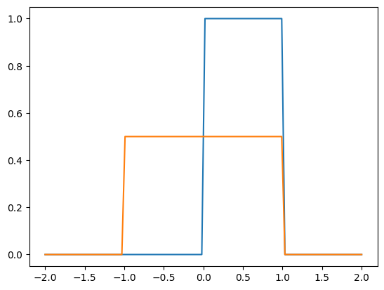
import matplotlib.pyplot as plt

# all priors including samplers implement `log_prob`
x = jnp.linspace(-2, 2, 100)
plt.plot(x, jnp.exp(prior.log_density(x)))
plt.plot(x, jnp.exp(sampler.log_density(x)))
plt.show()

Markov Chains

It may be desirable to generate asymptotically unbiased samples for a true distribution \(p_{true}(x)\) that the sample approximates, \(p_\theta(x) \approx p_{true}(x)\). The simplest way to achieve this is using the independent Metropolis-Hastings (IMH) algorithm.

An interface similar to blackjax’s blackjax.irmh is provided in IMH. The main difference to blackjax is that here, the proposal probabilities are computed at the same time as the samples.

Markov chains inherently generate one sample at a time, while normalizing flows can naturally generate batches of samples. One option is of course to run multiple chains in parallel. Besides that, BufferedSampler wraps around a distribution and internally draws from a buffer when individual samples are requested, that is redrawn when the buffer is exhausted.

Parameter manipulation & freezing

Both distributions and bijections are nnx.Modules and contain variables.

In order to indicate constant arrays that are not to be updated in gradient descent, the Const class, which is a subclass of nnx.Variable, can be used.

It may also be useful to freeze some parameters of a bijection or distributions that have been trained before, but should now be considered “fixed”. One way to achieve this is demonstrated below.

fixed = bijx.Scaling(bijx.Const(2.0))

# split into graph, constants, and parameters
graph, const, params = nnx.split(fixed, bijx.FrozenFilter, nnx.Param)
print(f'{const=}\n{params=}')

const=State({
  'scale': {
    'param': Const(
      value=2.0
    )
  }
})
params=State({})

# by default, initialized as trainable parameter
trainable = bijx.Scaling((), rngs=nnx.Rngs(params=0))

graph, const, params = nnx.split(trainable, bijx.FrozenFilter, nnx.Param)
print(f'{const=}\n{params=}')

const=State({})
params=State({
  'scale': {
    'param': Param( # 1 (4 B)
      value=Array(1., dtype=float32)
    )
  }
})

Now for convenience, we can wrap bijections in the bijx.Frozen class, marking all sub-parameters as constant.

frozen = bijx.Frozen(trainable)
graph, const, params = nnx.split(frozen, bijx.FrozenFilter, nnx.Param)
print(f'{const=}\n{params=}')

const=State({
  'frozen': {
    'scale': {
      'param': Param( # 1 (4 B)
        value=Array(1., dtype=float32)
      )
    }
  }
})
params=State({})