Gaussian Mixture Model Training on Spiral Data

This tutorial demonstrates how to train a diagonal Gaussian mixture model on spiral data using forward KL divergence (maximum likelihood estimation). This serves as a basic training example showing the core patterns used in bijx for training probability distributions.

Unlike the continuous flow examples, this tutorial focuses on directly training a parametric distribution (GMM) without bijective transformations, making it a good starting point for understanding the training patterns in bijx. The model can easily be replaced or extended with further bijection layers.

import flax.nnx as nnx
import jax
import jax.numpy as jnp
import matplotlib.pyplot as plt
import numpy as np
import optax
from tqdm import tqdm

import bijx

# define a random number sequence for convenience
rngs = nnx.Rngs(0)

Data Generation

First, let’s create a function to generate 2D spiral data. This will serve as our target distribution that we want the GMM to learn.

def generate_spiral_data(n_samples=1000, noise=0.02, seed=42):
    """Generate 2D spiral data."""
    rng = np.random.RandomState(seed)
    t = 5 * rng.rand(n_samples) * np.pi
    x = t * np.cos(t) / 20
    y = t * np.sin(t) / 20
    # Add noise
    x += noise * rng.randn(n_samples)
    y += noise * rng.randn(n_samples)
    return jnp.stack([x, y], axis=1)

def plot_data_and_model(data, model, title="Data and Model", figsize=(12, 4)):
    """Plot the data and model density/samples."""
    plt.figure(figsize=figsize)

    # Plot original data
    plt.subplot(1, 3, 1)
    plt.scatter(data[:, 0], data[:, 1], alpha=0.5, s=10)
    plt.title("Original Data")
    plt.xlabel("x")
    plt.ylabel("y")
    plt.axis('equal')

    # Plot model samples
    plt.subplot(1, 3, 2)
    samples, _ = model.sample(batch_shape=(len(data),))
    plt.scatter(samples[:, 0], samples[:, 1], alpha=0.5, s=10, color='orange')
    plt.title("Model Samples")
    plt.xlabel("x")
    plt.ylabel("y")
    plt.axis('equal')

    # Plot model density
    plt.subplot(1, 3, 3)
    # Create grid for density evaluation
    x_range = [data[:, 0].min() - 0.5, data[:, 0].max() + 0.5]
    y_range = [data[:, 1].min() - 0.5, data[:, 1].max() + 0.5]
    x_grid, y_grid = jnp.mgrid[
        x_range[0]:x_range[1]:100j,
        y_range[0]:y_range[1]:100j
    ]
    grid_points = jnp.stack([x_grid.ravel(), y_grid.ravel()], axis=1)

    # Evaluate density
    log_densities = model.log_density(grid_points).reshape(x_grid.shape)

    plt.imshow(
        log_densities.T,
        extent=[x_range[0], x_range[1], y_range[0], y_range[1]],
        origin='lower',
        aspect='auto',
        cmap='viridis'
    )
    plt.colorbar(label='Log density')
    plt.title("Model Density")
    plt.xlabel("x")
    plt.ylabel("y")

    plt.suptitle(title)
    plt.tight_layout()
    plt.show()

Configuration and Data Generation

Let’s set up our training configuration and generate the spiral data.

# Configuration
n_components = 64
n_samples = 1000
n_epochs = 50  # Reduced for faster execution
batch_size = 128
learning_rate = 1e-2

# Generate spiral data
data = generate_spiral_data(n_samples=n_samples, noise=0.02, seed=42)
print(f"Data shape: {data.shape}, range: [{data.min():.2f}, {data.max():.2f}]")

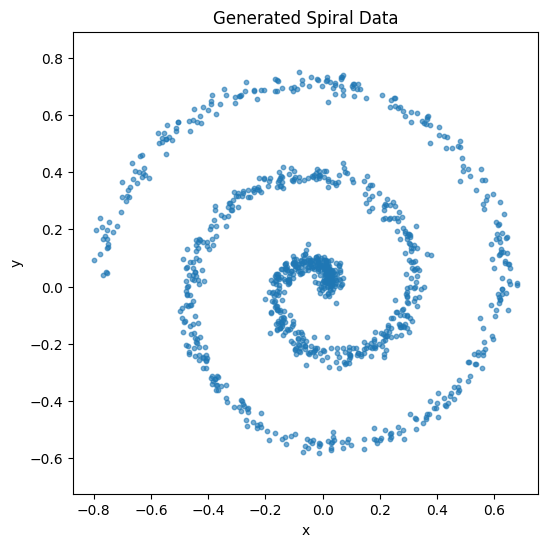
# Visualize the data
plt.figure(figsize=(6, 6))
plt.scatter(data[:, 0], data[:, 1], alpha=0.6, s=10)
plt.title("Generated Spiral Data")
plt.xlabel("x")
plt.ylabel("y")
plt.axis('equal')
plt.show()

Data shape: (1000, 2), range: [-0.80, 0.75]

Model Creation

Now let’s create the diagonal Gaussian mixture model using the new GaussianMixture class from bijx. We’ll initialize the component means, variances, and mixture weights.

# Create diagonal Gaussian mixture model
print(f"Creating diagonal GMM with {n_components} components...")

# Initialize means and variances for the mixture components
means_init = jax.random.normal(rngs(), (n_components, 2)) * 0.5
scales_init = jnp.ones((n_components, 2)) * 0.5
weights_init = jnp.zeros(n_components)  # Will be normalized via softmax

# Create the Gaussian mixture model
gmm = bijx.GaussianMixture(
    means=means_init,
    covariances=scales_init**2,  # DiagonalNormal expects variances
    weights=weights_init,
    rngs=rngs
)

print(f"Model created with {n_components} components")
print(f"Initial means shape: {means_init.shape}")
print(f"Initial scales shape: {scales_init.shape}")

Creating diagonal GMM with 64 components...
Model created with 64 components
Initial means shape: (64, 2)
Initial scales shape: (64, 2)

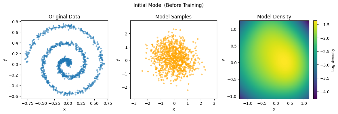
# Plot initial model
plot_data_and_model(data, gmm, "Initial Model (Before Training)")

Training Setup

Now let’s set up the optimization. We’ll use forward KL divergence (maximum likelihood) as our objective, which means we want to minimize the negative log-likelihood of the data under our model.

The loss function is: \(L = -\mathbb{E}_{x \sim \text{data}}[\log p_{\theta}(x)]\)

where \(p_{\theta}(x)\) is our GMM density.

# Set up optimization
optimizer = nnx.Optimizer(
    gmm,
    optax.adam(learning_rate),
    wrt=nnx.Param,
)

@nnx.jit
def training_step(model, optimizer, batch):
    """Single training step using forward KL (maximum likelihood)."""
    def loss_fn(model):
        # Forward KL: minimize -log p(x) = minimize negative log-likelihood
        log_probs = model.log_density(batch)
        return -jnp.mean(log_probs)

    loss, grads = nnx.value_and_grad(loss_fn)(model)
    optimizer.update(grads=grads, model=model)
    return loss

Training Loop

Now let’s run the training loop. We’ll use mini-batch stochastic gradient descent with shuffling.

# Training loop
print(f"Starting training for {n_epochs} epochs...")
print(f"Batch size: {batch_size}")
print(f"Learning rate: {learning_rate}")

losses = []
n_batches = len(data) // batch_size

# Create batches
key = jax.random.PRNGKey(42)

for epoch in tqdm(range(n_epochs), desc="Training"):
    epoch_losses = []

    # Shuffle data each epoch
    key, subkey = jax.random.split(key)
    indices = jax.random.permutation(subkey, len(data))
    shuffled_data = data[indices]

    # Process batches
    for i in range(n_batches):
        batch_start = i * batch_size
        batch_end = min((i + 1) * batch_size, len(data))
        batch = shuffled_data[batch_start:batch_end]

        loss = training_step(gmm, optimizer, batch)
        epoch_losses.append(loss)

    avg_loss = jnp.mean(jnp.array(epoch_losses))
    losses.append(avg_loss)

    # Print progress occasionally
    if (epoch + 1) % 10 == 0 or epoch == 0:
        print(f"Epoch {epoch + 1:3d}: Loss = {avg_loss:.4f}")

print(f"\nTraining completed! Final loss: {losses[-1]:.4f}")

Starting training for 50 epochs...
Batch size: 128
Learning rate: 0.01

Training: 100%|██████████| 50/50 [00:00<00:00, 121.62it/s]

Epoch   1: Loss = 1.4185
Epoch  10: Loss = 0.2768
Epoch  20: Loss = -0.2451
Epoch  30: Loss = -0.4850
Epoch  40: Loss = -0.5821
Epoch  50: Loss = -0.6005

Training completed! Final loss: -0.6005

Results and Analysis

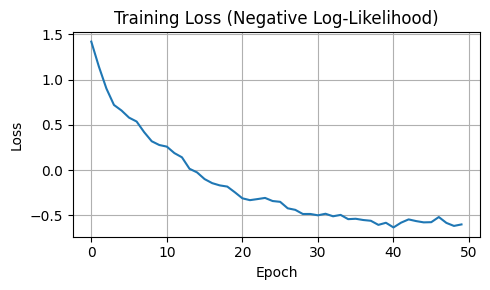
Let’s analyze the training results by plotting the loss curve and examining the final model.

# Plot training progress
plt.figure(figsize=(5, 3))
plt.plot(losses)
plt.title("Training Loss (Negative Log-Likelihood)")
plt.xlabel("Epoch")
plt.ylabel("Loss")
plt.grid(True)

plt.tight_layout()
plt.show()

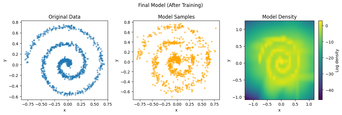
# Show final results
plot_data_and_model(data, gmm, "Final Model (After Training)")