Continuous flows

A continuous (normalizing) flow transforms a base distribution \(p_0(x_0)\) into a target distribution \(p_T(x_T)\) by evolving samples along the solution of an ODE:

\[ \frac{dx}{dt} = f(t, x), \quad x(0) = x_0, \quad x(T) = x_T \,. \]

The key insight is that the log-density evolves according to the instantaneous change of variables formula:

\[ \frac{d \log p(x(t))}{dt} = -\nabla_x \cdot f(t, x(t)) = -\sum_{i=1}^d \frac{\partial f_i}{\partial x_i} \,. \]

This gives us the augmented ODE system that bijx implements:

\[\begin{split} \begin{aligned} \frac{dx}{dt} &= f(t, x) \\ \frac{d \log p}{dt} &= -\nabla_x \cdot f(t, x) \,. \end{aligned} \end{split}\]

The solution of this ODE defines a transformed distribution \(p_T(x_T)\).

Vector Fields and Solvers

The approach taken in bijx is to split the problem into two components: the vector field, and the solver. Most effort of defining a normalizing flow architecture then goes into the vector field. All continuous flows in bijx expect vector fields with the signature:

def vector_field(t: float, x: Array, **kwargs) -> Tuple[Array, Array]:
    """
    Args:
        t: Time parameter
        x: Current state
        **kwargs: Additional arguments (e.g., conditioning)

    Returns:
        dx_dt: Time derivative of state
        dlogp_dt: Time derivative of log-density
    """
    # schematically
    dx_dt = neural_network(t, x, **kwargs)
    dlogp_dt = -divergence(dx_dt, x)  # Negative divergence
    return dx_dt, dlogp_dt

This may typically be implemented by an nnx.Module class which has a __call__ method with this signature.

Two types of solvers are implemented that turn this vector field into a bijection: ContFlowDiffrax and ContFlowRK4. For most applications ContFlowDiffrax is likely the best choice, as it wraps around the powerful diffrax library for ODE solving.

Both are subclasses of Bijection and implement the forward and reverse defined by integrating the vector field forward/backward. Thus, once a vector field is converted into a bijection, it can be used just as any other bijection, including chaining them together, and defining new distributions as samplers.

import jax.numpy as jnp
from flax import nnx
import diffrax
import bijx


# Basic example, with a dummy vector field on a scalar `x`

class DummyVectorField(nnx.Module):

    def __call__(self, t, x, **kwargs):
        center = 0.5
        # repel samples from center of [0, 1]
        dx_dt = (x - center)**3
        # divergence
        dlogp_dt = -3*(x - center)**2
        return dx_dt, dlogp_dt


cnf = bijx.ContFlowDiffrax(
    vf=DummyVectorField(),
    # exposes arguments of diffrax.diffeqsolve
    config=bijx.DiffraxConfig(
        # start and end time for flow
        t_start=0.0,
        t_end=1.0,
        # initial step size
        dt=0.1,
        # solver, and adaptive step size controller
        solver=diffrax.Dopri5(),
        stepsize_controller=diffrax.PIDController(atol=1e-5, rtol=1e-5),
        # adjoint; can set to diffrax.BacksolveAdjoint() if memory constrained
        adjoint=diffrax.RecursiveCheckpointAdjoint(),
    )
)

# define a sampler, by transforming the uniform distribution with the flow

sampler = bijx.Transformed(
    bijx.IndependentUniform(event_shape=(), rngs=nnx.Rngs(0)),
    cnf,
)

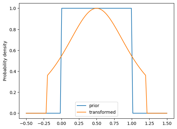
import matplotlib.pyplot as plt

xs = jnp.linspace(-0.5, 1.5, 100)
ld = sampler.prior.log_density(xs)
plt.plot(xs, jnp.exp(ld), label='prior')

ld = sampler.log_density(xs)
plt.plot(xs, jnp.exp(ld), label='transformed')

plt.ylabel('Probability density')

plt.legend()
plt.show()

Autodiff Jacobian

Esepcially in higher-dimensional cases, it is important to design the vector field architecture such that efficient divergence computation can be implemented, if this is used to compute the log-density change. However, in lower-dimension and for prototyping, it may be sufficient to use JAX’s automatic differentiation to compute the Jacobian. For convenience this is implemented in AutoJacVF. It wraps a vector field (callable) that only returns \(dx/dt\) and converts it into a new vector field that also returns the negative divergence (trace of the Jacobian).

def two_dim_vf(t, x):
    # some two dimensional vector field
    return jnp.sin(x) + jnp.cos(x[..., ::-1])

# event_dim=1 indicates x is a vector (one event dimension)
vf = bijx.AutoJacVF(two_dim_vf, event_dim=1)

# now returns both dx/dt and -tr(jac)
# this vf can be used to define a continuous flow as above
vf(0, jnp.array([1.0, 2.0]))

(Array([0.4253241, 1.4495997], dtype=float32),
 Array(-0.12415543, dtype=float32))