Analytic Bijections

This tutorial demonstrates how to leverage the analytic bijections defined in bijx, first in 1D and then in new radial flows in 2D.

from flax import nnx
import jax
import jax.numpy as jnp
import optax
import numpy as np
import matplotlib.pyplot as plt
from tqdm import tqdm

import bijx

rngs = nnx.Rngs(0)

1D Example

We can learn onedimensional distributions by stacking sufficiently many scalar bijections. First, we’ll define a synthetic target distribution as an example.

@nnx.dataclass
class PolyTarget:
    # Oscillatory Gaussian component coefficients
    a1: nnx.Data[float] = 1.0  # Amplitude of sin term
    w1: nnx.Data[float] = 5.0  # Frequency of sin
    g1: nnx.Data[float] = 5.0  # Gaussian decay rate

    # Cosine component
    a2: nnx.Data[float] = 2.0  # Amplitude of cos term
    w2: nnx.Data[float] = 10.0  # Frequency of cos

    # Polynomial component
    a4: nnx.Data[float] = -0.2

    def __call__(self, x):
        """Compute unnormalized log density."""
        # Handle both (batch,) and (batch, 1) shapes
        x_flat = x.squeeze(-1) if x.shape[-1] == 1 else x

        log_p = (
            self.a1 * jnp.sin(self.w1 * x_flat) * jnp.exp(-self.g1 * x_flat**2)
            + self.a2 * jnp.cos(self.w2 * x_flat)
            + self.a4 * x_flat**4
        )
        return log_p

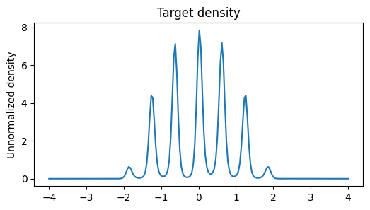
poly_target = PolyTarget()

plt.figure(figsize=(6, 3))
plt.title('Target density')
x = jnp.linspace(-4, 4, 200)
plt.plot(x, jnp.exp(poly_target(x)))
plt.ylabel('Unnormalized density')
plt.show()

Model

Instead of a for-loop over multiple bijections, we use bijx.ScanChain which chains the internal bijection using jax’s scan. The internal bijection is expected to have parameters with leading batch dimension, which is achieved by applying vmap over a number of random keys.

stack_size = 64

@nnx.split_rngs(splits=stack_size)
@nnx.vmap(in_axes=(0,), out_axes=0)
def create_bijection_stack(rngs):
    # base = bijx.SinhConjugation(rngs=rngs)
    # base = bijx.CubicRational(rngs=rngs)

    base = bijx.CubicConjugation(rngs=rngs)

    return bijx.ScanChain(base)

bijection = create_bijection_stack(nnx.Rngs(0))
model = bijx.Transformed(
    bijx.IndependentNormal((), rngs=nnx.Rngs(0)),
    bijection,
)

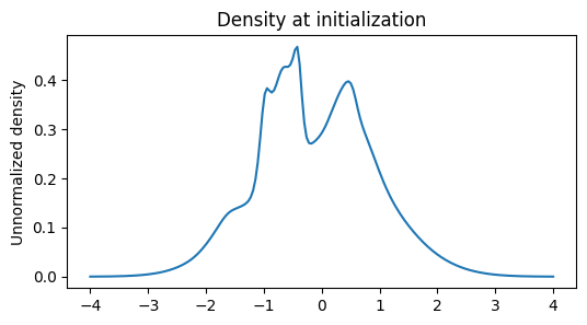
plt.figure(figsize=(6, 3))
plt.title('Density at initialization')
x = jnp.linspace(-4, 4, 200)
plt.plot(x, jnp.exp(model.log_density(x)))
plt.ylabel('Unnormalized density')
plt.show()

Training

# simple training setup
batch_size = 256

optimizer = nnx.Optimizer(
    tx=optax.adam(1e-3),
    model=model,
    wrt=nnx.Param,
)

def loss_fn(model):
    x, lq = model.sample((batch_size,))
    lp = poly_target(x)
    return -jnp.mean(lp - lq)

@nnx.jit
def update_step(model, optimizer):
    loss, grads = nnx.value_and_grad(loss_fn)(model)
    optimizer.update(grads=grads, model=model)
    return loss

steps = 2000
losses = np.full(steps, np.nan)

for i in tqdm(range(steps)):
    losses[i] = update_step(model, optimizer)

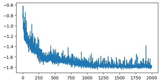
plt.figure(figsize=(6, 3))
plt.plot(losses)
plt.xlabel('Step')
plt.ylabel('Loss')
plt.show()

100%|██████████| 2000/2000 [00:05<00:00, 341.69it/s]

[<matplotlib.lines.Line2D at 0x1178bf0e0>]

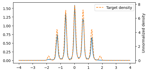
Evaluation

plt.figure(figsize=(6, 3))
x = jnp.linspace(-4, 4, 200)
plt.plot(x, jnp.exp(model.log_density(x)), label='Learned density')
plt.twinx()
plt.plot(x, jnp.exp(poly_target(x)), '--', label='Target density', color='C1')
plt.ylabel('Unnormalized density')
plt.legend()
plt.show()

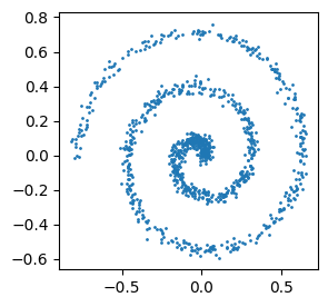
Radial flows

First we define a spiral distribution in 2D, this time by defining how to sample from it.

Target

@nnx.dataclass
class SpiralData:

    n_turns: nnx.Data[float] = 2.5  # Number of spiral turns (5 * pi / (2 * pi) = 2.5)
    radius_scale: nnx.Data[float] = 1.0 / 20.0  # Scaling factor for spiral radius
    noise_scale: nnx.Data[float] = 0.02  # Gaussian noise added to spiral
    is_normalized: bool = False  # No density, so not normalized

    @property
    def event_shape(self) -> tuple[int, ...]:
        return (2,)

    def sample(self, batch_shape: tuple[int, ...] = (), *, rng):
        """Generate spiral samples using JAX-compatible operations."""
        total_samples = int(np.prod(batch_shape))

        # Generate parameter t uniformly from 0 to n_turns * 2 * pi
        rng1, rng2 = jax.random.split(rng)
        t = jax.random.uniform(rng1, (total_samples,), minval=0, maxval=self.n_turns * 2 * jnp.pi)

        # Generate spiral coordinates
        x = t * jnp.cos(t) * self.radius_scale
        y = t * jnp.sin(t) * self.radius_scale

        # Add Gaussian noise
        noise = jax.random.normal(rng2, (total_samples, 2)) * self.noise_scale

        # Combine and reshape
        samples = jnp.stack([x, y], axis=1) + noise
        return samples.reshape(*batch_shape, 2)

spiral_data = SpiralData()

samples = spiral_data.sample((1000,), rng=jax.random.key(0))
plt.figure(figsize=(3, 3))
plt.scatter(samples[:, 0], samples[:, 1], s=1)
plt.show()

Model architecture

First, we now want to transfrom radii, with respect to some trainable center. Thus, we must make sure that we map rays onto rays (i.e. preserve origin).

stack_size = 64

@nnx.split_rngs(splits=stack_size)
@nnx.vmap(in_axes=(0,), out_axes=0)
def create_bijection_stack(rngs):
    # base = bijx.SinhConjugation(rngs=rngs)
    # base = bijx.CubicRational(rngs=rngs)
    base = bijx.CubicConjugation(rngs=rngs)

    # now wrapped in ray transform
    return bijx.RayTransform(bijx.ScanChain(base))

We will use a simple Fourier-series based coupling layer to make the radial transformation depend on the angle.

class FourierCondNet(nnx.Module):
    """Fourier-based conditioning network for angle-dependent parameters."""

    def __init__(
        self,
        output_dim: int,
        fourier_count: int = 3,
        hidden_dim: int | None = None,
        *,
        rngs: nnx.Rngs,
    ):
        assert fourier_count % 2 == 1, 'Fourier count must be odd'
        self.kernel = bijx.nn.embeddings.KernelFourier(
            fourier_count, val_range=(-jnp.pi, jnp.pi)
        )
        self.output_dim = output_dim

        if hidden_dim is not None:
            self.hidden = nnx.Linear(
                fourier_count, hidden_dim,
                use_bias=False, rngs=rngs,
                kernel_init=nnx.initializers.normal(0.01),
            )
            final_in = hidden_dim
        else:
            final_in = fourier_count

        self.superpos = nnx.Linear(
            final_in, output_dim,
            use_bias=False, rngs=rngs,
            kernel_init=nnx.initializers.normal(0.01),
        )

    def __call__(self, x_hat):
        """Map unit vectors to bijection parameters.

        Args:
            x_hat: Unit vectors of shape (..., 2).

        Returns:
            Parameters of shape (..., output_dim).
        """
        theta = jnp.atan2(x_hat[..., 1], x_hat[..., 0])
        features = self.kernel(theta)

        # Regularize feature magnitudes: suppress high frequencies
        freq_count = (self.kernel.feature_count - 1) // 2
        freq_indices = jnp.concatenate([
            jnp.arange(1, freq_count + 1),  # for sin terms
            jnp.arange(1, freq_count + 1),  # for cos terms
            jnp.array([1.0])  # for constant term
        ])
        features = features / freq_indices

        if hasattr(self, 'hidden'):
            features = self.hidden(features)
        return self.superpos(features)

def create_radial_layer(rngs):
    base = create_bijection_stack(rngs)

    cond_net = FourierCondNet(
        output_dim=bijx.ModuleReconstructor(base).params_total_size,
        fourier_count=7,
        rngs=rngs
    )

    layer = bijx.RadialConditional(
        scalar_bijection=base,
        cond_net=cond_net,
        center=jnp.array([-0.5, -1.]),
        scale=jnp.zeros(2),
        rngs=rngs
    )

    return layer

model = bijx.Transformed(
    bijx.IndependentNormal((2,), rngs=rngs),
    create_radial_layer(rngs)
)

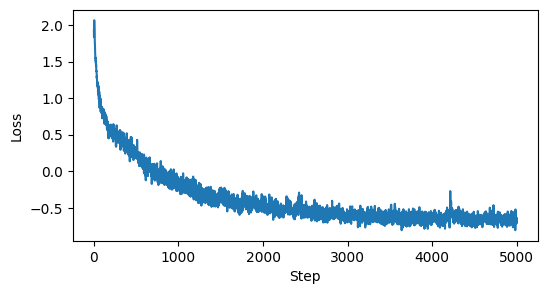
Training

# simple training setup
batch_size = 512

optimizer = nnx.Optimizer(
    tx=optax.adam(1e-2),
    model=model,
    wrt=nnx.Param,
)

def loss_fn(model):
    x = spiral_data.sample((batch_size,), rng=model.rngs())
    lq = model.log_density(x)
    return -jnp.mean(lq)

@nnx.jit
def update_step(model, optimizer):
    loss, grads = nnx.value_and_grad(loss_fn)(model)
    optimizer.update(grads=grads, model=model)
    return loss

steps = 5000
losses = np.full(steps, np.nan)

for i in tqdm(range(steps)):
    losses[i] = update_step(model, optimizer)

plt.figure(figsize=(6, 3))
plt.plot(losses)
plt.xlabel('Step')
plt.ylabel('Loss')
plt.show()

100%|██████████| 5000/5000 [00:33<00:00, 148.29it/s]

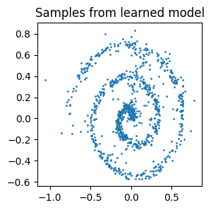
Evaluation

x, _ = model.sample((1000,))
plt.figure(figsize=(3, 3))
plt.title('Samples from learned model')
plt.scatter(x[:, 0], x[:, 1], s=1)
plt.show()